Main Ideas from this Post

1. An understanding of the theoretical connections between compression and induction.
2. A sense that large language models likely do not (yet) qualify as general-compression algorithms; thus are "far" from performing universal induction.
3. A series of jumping-off points for further research in this area, including the measuring of a model's compression capabilities via latent representation sizes in a manner inspired by Shannon information theory.

There is also a wonderful introduction to Solomonoff Induction by Eliezer Yudkowsky in the style of an A-B dialogue. I highly recommend it for all.

Mathematical Background

We place ourselves in a situation familiar to any machine learning model undergoing training: given some observed data, come up with a prediction method or theory that is both (1) consistent with the observations and (2) as perfect a predictor as possible on future instances.

Glossary

Before stating any theorems, we provide a quick glossary:

• Induction/Inductive Inference: the process of reassigning a likelihood to a theory having observed particular instances. "Determining the truth."
  • All inference problems can be cast in the form of extrapolation (i.e., continuation) from an ordered sequence of binary symbols; think of this as a standard form.
• Epicurus' Principle of Multiple Explanations: (paraphrased as) Any and all theories consistent with all observations ought to be considered (but not necessarily with equal consideration).
  • Any such theory is also called a hypothesis.
• Occam's Razor Principle: (paraphrased as) Among the theories that are consistent with all observations, one should prefer the simplest.
• Computable: any operation or object which can be simulated by a Turing machine (or computer program in some Turing-complete programming language).
• Lossless Compression: the process of representing information in a more compact form in such a way that the process is perfectly invertible.
• Kolmogorov Complexity: the simplicity of a theory or object can be measured by the shortest length computer program describing* that theory or object. I.e., by the amount of information in the theory or object that is impossible to computably, losslessly compress further.
  • (*) To describe a thing is to produce a description of it; i.e., to produce a code such that a fixed universal decoder could perfectly recuperate the original thing from that code.
  • A special type of Kolmogorov complexity — known as monotone complexity and denoted by \(\text{Km}(\cdot)\) — is defined similarly except using only monotone Turing machines, or those which cannot change their mind about previous predictions when given new observations.
• Minimum Description Length (MDL) Principle: the Occam-type principle declaring the most preferable hypothesis to be that which has (1) the simplest theory and (2) the simplest description of the observations from that theory (as measured by Kolmogorov complexity).
• Bayes' Rule: a mathematical law to update likelihoods of various hypotheses given some observations based on conditional probability.
• Solomonoff Induction (SI): a method of "perfect" induction which performs sequence prediction using a weighted-combination of the consistent theories weighted by their complexities and using Bayes' Rule to update the hypotheses' likelihoods upon new observations; it presumes that the stochastic process generating the data is governed by a (somewhat) computable prior probability distribution. SI fulfills the metaphysical principles of Epicurus and MDL.
• Universal prior distribution: a somewhat computable (i.e., lower semi-computable, or approximable by a Turing machine from below), continuous semi-measure (i.e., distribution of likelihoods on all possible theories given some data that doesn't necessarily sum fully to \(100\%\)) which can essentially play the role of any prior distribution on theories in Solomonoff Induction without much sacrifice.

Fact 1: There exists a universal prior distribution.

This fact is one of the key reasons Solomonoff Induction is even possible. For any other (computable) priori distribution \(P\) one might place on the set of consistent hypotheses to the observed data, this universal prior distribution \(\mathbf{M}\) has the property that there is some multiplicative constant \(\alpha > 0\) such that for any hypothesis \(H\) and observed data \(D\),

\[\mathbf{M}(H \mid D) > \alpha \cdot P(H \mid D).\]

That is, the universal prior assigns at least a certain, guaranteed proportion of the mass that the arbitrary prior \(P\) does to all hypotheses.

Fact 2: Perfect induction can be done even if we take the same universal prior distribution as our prior anytime we wish to perform induction on data generated by a computable underlying process. (See Theorem 5.2.2 of Li and Vitányi).

Great! so let's just code up Solomonoff Induction:

def Solomonoff_Induction(data):
	universal_priori_distribution = ...

Fact 3: No universal prior distribution can be computable. Therefore, there is no algorithm (hand-coded or machine-learned, alike) which can simulate the values of this distribution.

It is for this reason that we cannot finish writing that algorithm above, and further that Solomonoff Induction is impossible to perfectly follow by anyone or anything that thinks like a computer.

It is important to note here that there is a relationship between the universal prior distribution and Kolmogorov complexity. Lemma 4.5.6 of Li and Vitányi can be interpreted as saying the following.

Fact 4: In the limit of more observational data \(D\), the universal prior distribution assigns the hypothesis \(H\) (hypothesizing the values of the next few observations) an updated likelihood whose value is related to the monotone complexities of the data \(D\) and the concatenation \(DH\) of data \(D\) and hypothesis \(H\):
\[\mathbf{M}(H \mid D) = \frac{\mathbf{M}(DH)}{\mathbf{M}(D)} \approx 2^{\text{Km}(D) - \text{Km}(DH)}.\]

Now we can unveil the use of compression in prediction: if \(P\) is any probability distribution on hypotheses/data (or, in particular, the exact one governing the data), then for almost any extrapolating hypothesis \(H\) which is sufficiently compressible from the data: i.e., satisfying \(\text{Km}(DH) \leq \text{Km}(D) + c\) for some constant value \(c > 0\), the probability of this hypothesis under \(P\) must satisfy \(P(H \mid D) > \beta \cdot2^{-c}\) for some \(\beta > 0\). In words,

Fact 5: It is a good heuristic to choose the extrapolating \(H\) that minimizes the length difference between the shortest program that outputs \(DH\) and the shortest program that outputs \(D\).

Generative Models as Compressors

Sometimes a boast and other times a criticism: machine learning performs exceptionally well for no good reason. Remember, any AI model is essentially a very complicated algorithm, and generative AI models are then very complicated prediction algorithms. As we have seen, being able to compress data very well is in some way equivalent to being able to extrapolate, predict, or induct on data very well.

So, in this sense, training impressive generative models is equivalent to training impressive compression algorithms. The "perfect" compression procedure would assign to each object the codeword being the shortest program returning that object; but just as the universal prior distribution \(\mathbf{M}\) is not computable, neither is the "perfect," universal compressor. This follows from Kolmogorov complexity not being computable. Worse yet, this function is so uncomputable that no algorithm can come close to agreeing with it in value on more than just a finite number of exceptional objects (see Theorem 2.3.2 of Li and Vitányi). So our computable machine learning models cannot hope to ever learn universal compression.

Despite this, that does not stop machine learning models from learning to compress very well and with minimal loss. In general, we’d expect any sufficiently large model to develop a system for compression that beats any standard, generic compression algorithm; this is a sort of convergence behavior.

Safety Implications

Large language models (LLMs) are trained to compress sequences while gaining knowledge about the world. There already exists research from 2023 demonstrating LLMs' capabilities in performing compression at a level comparable to standard, generic compression algorithms (See Delétang et al., 2023).

Still, it is largely unclear to what extent existing or imminent large language models have learned to perform compression. Understanding this difference has relevance in AI Safety: according to Grosse, 2024,

"[Aritificial Intelligence \(\times\) Induction (AIXI)], a simple model of superintelligent AGI… combines universal induction with optimal planning. The idea [is] that compression and sequential decision making are all you need for AGI…. From an alignment perspective, AIXI is a constructive proof of the Orthogonality Thesis: despite being extremely smart, it continues optimizing whatever silly objective you gave it. It's also really hard to specify goals directly because its internal representations are opaque.

LLMs are really good compressors, though (fortunately) we don't yet have good enough sequential decision making algorithms to build an AIXI-like agent.… Is [AIXI] a good model for the limit of GPT-\(k\) for large \(k\)? There are some suggestive similarities, but also some important differences (e.g. lots of background knowledge, limited sequential depth, lack of weight sharing → hard to express iterative computations, no directed information acquisition)."

The goal of this project is to investigate further the compression capabilities of generative models. Any results of such an investigation would serve as proxies for the inductive capabilities of the tested generative models. Should some GPT-\(k\) be capable of performing nearly perfect (Solomonoff) induction, humanity might come into contact with an exceptionally intelligent agent. Evidence in either direction speaks to what AI research must still overcome before reaching this AIXI state.

Experimentation

I propose two novel experiments to investigate the compression capabilities of generative models. The main ideas from each experiment are as follows:

• Experiment 1: Can GPT models perform compression well when you ask them to?
• Experiment 2: Are GPT models impressive because they learn to compress well?

Experiment 1: GPT Models as Compressors

Motivation

A shallow interpretation of our general research goal might be to ask the following question:

Question: Can ChatGPT perform nearly lossless compression in its I/O?

While the formal connections between compression and induction capabilities strictly refer to how a model internally represents data, this naïve question nevertheless deserves some thought: to what extent is training a model for natural language tasks also training a model to perform compression?

In particular, do large language models obey the typical laws of a complexity function or compressor? Let \(A: \texttt{Strings} \to \texttt{Strings}\) be a map on finite strings, \(\texttt{s} \in \texttt{Strings}\) be a finite string, and \(C(\texttt{s}) = \text{length}(A(\texttt{s}))\) the length of however \(A\) represents the string \(\texttt{s}\). Recall that in order for \(A\) to qualify as a lossless or injective compression algorithm, there must be a corresponding program \(A^{-1}\) computing the inverse of \(A\), i.e. such that \(A^{-1} \circ A \equiv \text{id}\). The following are various properties one might ask of a compression algorithm \(A\), where inequalities only hold up to an additional \(O(\log n)\) term, where \(n\) is the maximal length of a string involved in the concerned inequality. Formally, these are desiderata characterizing normal compressors.

• Idempotency: Compression is no harder for repetitive inputs:
  \[C(\texttt{s}, \texttt{s}) = C(\texttt{s}).\]
• Monotonicity: Compression is harder given more inputs:
  \[C(\texttt{s}) \leq C(\texttt{s}, \texttt{t}).\]
• Symmetry: Compression doesn't much mind the order of inputs:
  \[C(\texttt{s}, \texttt{t}) = C(\texttt{t}, \texttt{s}).\]
• Distributivity: Compressing using an intermediate string cannot improve compression:
  \[C(\texttt{s}, \texttt{t}) + C(\texttt{w}) \leq C(\texttt{s}, \texttt{w}) + C(\texttt{t}, \texttt{w}). \]

See Clustering by Compression by Cilibrasi and Vitányi for more background to normal compressors.

Hypothesis

Due to hallucination, training data, and the transformer architecture of large language models, it is unlikely that they possess a generic ability to losslessly compress input data upon output, especially data not coming from natural language tasks. I further hypothesize that certain desiderata of normal compressors are more likely to be met than others. Namely, idempotency, monotonicity, and symmetry might have more convincing evidence in our experiment than distributivity.

Experimental Design

I design an experiment to evaluate just how well a GPT model behaves as a normal compressor. For computational feasibility, I went with a GPT-2 model available through Hugging Face's transformers library. Of course, the same could be done for more advanced models.

Dataset

I use the first \(50\) documents from the 20 Newsgroups dataset. The following figure illustrates the distribution of character counts for all \(50\) of the test inputs.

Compression Methods

I first compare the original sizes of the documents, their sizes when compressed using GPT-2, and their sizes when compressed using gzip.

Property Adherence

For each property, I calculate the proportional difference between the left-hand side and right-hand side of the respective inequality, normalized by the maximum length of the inputs involved. This gives us a proportional difference between the left and right-hand sides of the four desirable inequalities stated above.

Python code for Experiment 1 is included in the end of the post.

Results

As evidenced in the figure below, gzip consistently achieves the smallest compression sizes, whereas GPT-2 achieves compression sizes typically between the original and gzip-compressed sizes. Qualitatively, these results are partially good evidence to say that a relatively small large language model can notice redundancies and represent strings in a more compact format. Still, any noticed redundancies will likely be "low-hanging fruit" performed by simple replacements rather than through complex reassignments.

The histograms for the four properties reveal the following:

• Idempotency: Most proportional differences are near zero, indicating good adherence.
• Monotonicity: Significant right-tail up to \(+0.5\), suggesting non-adherence for some inputs.
• Symmetry: Most proportional differences are near zero, indicating good adherence.

Distributivity: Centered around \(+0.1\) with broad spread, suggesting non-adherence for some inputs.

Conclusion

The GPT-2 model demonstrates a partial ability to compress textual data, though not as effectively as traditional gzip compression. The tests for compression properties show varying levels of adherence:

• Idempotency and Symmetry: GPT-2 compression largely adheres to these properties;
  • GPT-2 is thus already compressing intelligently enough to not struggle encoding multiple copies of a single piece — nor permutations of multiple pieces of — data with much issue.
• Monotonicity and Distributivity: GPT-2 compression significantly deviates from these properties.
  • GPT-2 is thus not compressing well enough to take advantage of the mutual information between pieces of data. This is a fundamental obstacle to performing good compression.

Overall, while GPT-2 exhibits some compression capabilities, it does not fully comply with the expected properties of a normal, lossless compressor. Measuring any deviations from these properties serves as a sanity-check before claiming a large language model can perform lossless compression.

Experiment 2: GPT Latent Representations

Motivation

OpenAI's GPT models, such as ChatGPT, offer impressive language generation features.

Question: Have GPT models necessarily been optimized to compress inputs across their layers very well?

First: a sanity check.

It might come as no surprise that autoencoders trained on stock images are capable of compressing images better than a general-purpose compression algorithm (say, gzip). Equivalently, autoencoders must internally represent data in an economical yet minimally-lossy manner. Autoencoders consist of two main components: (1) an encoder that compresses the input data into a lower-dimensional latent representation and (2) a decoder that reconstructs the original data from this compressed form. This encoder-decoder framework mirrors the process of data compression and decompression, making autoencoders particularly suited for this task. Autoencoders — as neural networks — can capture complex, nonlinear relationships within the data due to their use of nonlinear activation functions.

I have constructed the following toy example to provide some grounds for our motivation behind Experiment 2. On the Fashion MNIST dataset, which consists of \(28 \times 28\) grayscale images of fashion items, I trained a convolutional autoencoder, which includes multiple convolutional and transposed convolutional layers for encoding and decoding the images, respectively. I ran the training for \(20\) epochs against a Mean Squared Error (MSE) loss function with Adam optimizer and learning rate \(0.001\). As the encoder compresses the input images into a latent representation and the decoder reconstructs the images from this compressed representation, I aimed to measure the sizes of precisely these latent representations. With a final loss of \(0.56\) (indicating some basic ability to reconstruct input images with some degree of accuracy), I computed the following representation sizes.

So, the convolutional autoencoder effectively compresses the image data, reducing the size to \(290\) bytes on average compared to \(545\) bytes achieved by gzip on average.

Visualizing the reconstructed images shows that the autoencoder captures the overall structure and global features of the original images. However, finer details and high-frequency information are often lost, resulting in somewhat blurred reconstructions.

Clearly, whatever form of compression the trained autoencoder performs is lossy, particularly in the realm of high-frequency details.

OpenAI does not natively provide a straightforward API to directly access intermediate hidden states or latent representations. So estimating representation size internally to some OpenAI GPT model as an external researcher would not be very straightforward. Hugging Face's transformers library allows one to load even more complex of pre-trained models and to access their hidden states. I would have liked to perform a similar investigation as above to deeper architectures, but actually was incapable of getting a single one of my implementations for this experiment to run on my machine due to computational infeasibility. Without results, what follows is a proposal for designing an informative experiment on existing large language models.

Ultimately, we wish to compare the latent GPT representation sizes of certain textual inputs with their original and standardly-compressed counterparts. How might one measure the size of the internal representation of a piece of data within a GPT model?

Within each of the model's feed-forward hidden layers are neuron activations which might be viewed as representations of the input to the model. One might take the number of neurons used in such as a layer as a quantity representing the size of one of the ways in which the model represents the input. But there are a few issues with this view:

• Layers come in many sizes and contain neurons whose activations take on values in a (approximately) continuous domain. Unlike counting the number of bytes in a string or bits in a binary string, it is not so straightforward to assign a size to a finite list of activations.
• Layer sizes are fixed by an architectural choice, so it does not seem reasonable to take the, say, minimal layer size as a measure for the size of the model's latent representation of a piece of data.
• Some neurons from the same layer should be more relevant to representing an input than others.

What might we do to circumvent these issues?

• One might gauge relevance by a perturbation analysis: does making a small change to the input significantly alter the value of a particular neuron's activation? Better yet, we could even quantify relevance as a partial derivative: what is the change in the neuron's activation \(\Delta a\) under the input perturbation \(\Delta x\)? It seems more reasonable to measure the model's latent representation of data \(x\) by only those neurons deemed relevant to representing \(x\).
• Even further: one might measure the size of a model's latent representation of data \(x\) at a particular layer as follows.

First an analogy: suppose our model is the identity function mapping every input string \(x \mapsto x\) to itself. Imagine \(x\) being some binary string of length \(n\); e.g., \(x = \underbrace{0100 \cdots 11}_{\text{length } n}\). Equivalently, \(x\) is a dyadic rational number with the binary expansion \(0.0100 \cdots 11\) (just precede the binary string form of \(x\) by a \(``0."\)). Then our model represents each binary string of length \(n\) in a uniformly-spaced distribution where each string is of distance at least \(\frac{1}{2} \cdot2^{-n}\) from any other representation. We might say, then, that the model provides each string of length \(n\) a representation of size \[-\log_2(\frac{1}{2} \cdot2^{-n}) = n - 1,\] since any perturbation less than distance \(2^{-(n-1)}\) to \(x\) will produce an output whose closest output representation amongst strings of length \(n\) is that of \(x\).

In general, for given input \(x\) and string of length \(n\), we might say the mass of \(x\)'s representation at layer \(\ell\) is the "direct weight" of all "perturbations" or strings \(y\) whose activations \(\ell(y)\) lies closest to \(\ell(x)\) compared to the activation \(\ell(\sigma)\) for any other string \(\sigma\) of length \(n\). Collect all such \(y\) into the set \(\ell^{-1}(x)\): \[\ell^{-1}(x) := \set{y \in \texttt{Strings}: x=\argmin_{\vert \sigma \vert = n} \set{\vert \vert \ell(\sigma) - \ell(y)\vert \vert_2}},\] and compute the direct weight of a set \(A\) of strings in some alphabet of size \(k\) as follows: \[\operatorname{DW}(A) = \sum_{\sigma \in A} k^{-\vert \sigma \vert}.\] Finally, declare the size of the latent representation of input \(x\) at layer \(\ell\) to be the quantity: \[- \operatorname{DW}(\ell^{-1}(x)) \log_k(\operatorname{DW}(\ell^{-1}(x))).\]

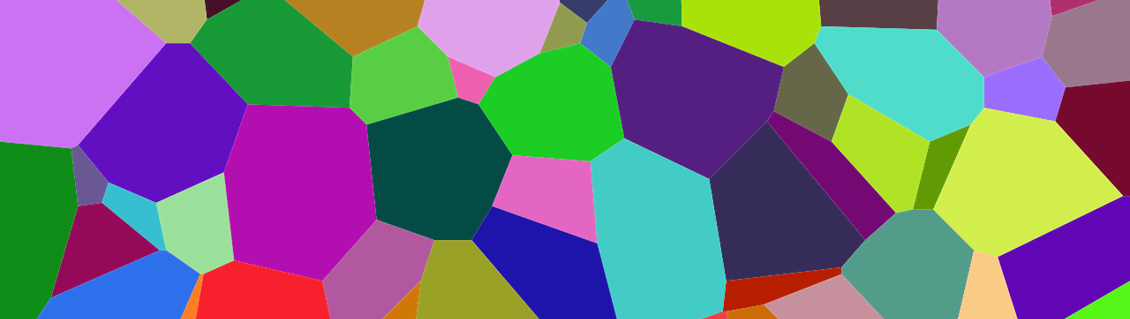
The motivation for this definition follows from the same reasoning as how one measures Shannon self-information of an input within a distribution: each outcome \(x\) of a random variable \(X\) has mass according to the probability \(\mathbb{P}(X = x)\) of the variable taking on that value. The Shannon self-information of that output is defined as \[- \mathbb{P}(X = x) \cdot \log \mathbb{P}(X = x),\] and the Shannon entropy of the random variable is just the expectation of the self-information across all possible outputs. In our situation, layer \(\ell\) of our model might bias its activation space to bunch together certain activations and leave other activations much sparser. The sparser the activation representations, the more weight this layer commits to the associated inputs, meaning it can compress the input to some extent. With this analogy in mind, we might call the final size of \(\ell\)'s representation of \(x\) the self-information of \(x\) under the length-\(n\) Voronoi distribution of \(\ell\). We imagine activation space broken into a Voronoi diagram, as illustrated below.

With this suggestion for estimating the latent representation size of data for a fixed model, one could straightforwardly compare this size to those of standard compression algorithms representations, just as I did in the toy example above.

References and Further Readings

• Cilibrasi, R., Vitányi, P. (2004). Clustering by compression. arXiv. https://arxiv.org/abs/cs/0312044.
• Delétang et al. (2023). Language modeling is compression. https://arxiv.org/abs/2309.10668.
• Grosse, R. (2024). Lecture 6: compression is all you need. In: CSC2547: AI Alignment. https://alignment-w2024.notion.site/Timelines-discussion-Universal-Induction-and-AIXI-417eef5b64d84382b27b2f696fcf2d08.
• Li, M., Vitányi, P. (2008). Inductive reasoning. In: An Introduction to Kolmogorov Complexity and Its Applications. Texts in Computer Science. Springer, New York, NY. https://doi.org/10.1007/978-0-387-49820-1_5.
• Vereshchagin, N., Shen, A. (2017). Algorithmic statistics: forty years later. https://arxiv.org/abs/1607.08077.
• Yudkowsky, E. (2015). Solomonoff induction: Intro Dialogue (Math 2). https://arbital.greaterwrong.com/p/solomonoff_induction/?l=1hh.

Appendix: Code for Experiment 1

import torch
from transformers import GPT2Tokenizer, GPT2LMHeadModel
from sklearn.datasets import fetch_20newsgroups
import gzip
import matplotlib.pyplot as plt

# Load pre-trained GPT-2 model and tokenizer
model_name = 'gpt2'
model = GPT2LMHeadModel.from_pretrained(model_name)
tokenizer = GPT2Tokenizer.from_pretrained(model_name)

# Set the pad_token to be the eos_token
tokenizer.pad_token = tokenizer.eos_token

# Compress text using GPT-2
def gpt_compress(text):
    inputs = tokenizer(text, return_tensors='pt', padding=True, truncation=True, max_length=512)
    attention_mask = inputs.attention_mask
    with torch.no_grad():
        outputs = model.generate(inputs.input_ids, attention_mask=attention_mask, max_length=inputs.input_ids.size(1) + 10, num_return_sequences=1, pad_token_id=tokenizer.eos_token_id)
    compressed = tokenizer.decode(outputs[0], skip_special_tokens=True)
    return compressed

# Measure compression size
def measure_size(text):
    return len(text.encode('utf-8'))

# Compress text using gzip and return the compressed size in bytes
def compress_gzip(text):
    compressed_file = 'compressed.gz'
    with gzip.open(compressed_file, 'wb') as f:
        f.write(text.encode('utf-8'))
    with open(compressed_file, 'rb') as f:
        compressed_data = f.read()
    return len(compressed_data)

# Testing various normal compressor properties

def test_idempotency(text):
    compressed_text = gpt_compress(text)
    compressed_text_twice = gpt_compress(compressed_text + ',' + compressed_text)
    lhs = measure_size(compressed_text_twice)
    rhs = measure_size(compressed_text)
    return (lhs - rhs) / measure_size(text)

def test_monotonicity(text1, text2):
    compressed_text1 = gpt_compress(text1)
    compressed_text_combined = gpt_compress(text1 + ',' + text2)
    lhs = measure_size(compressed_text1)
    rhs = measure_size(compressed_text_combined)
    return (rhs - lhs) / max(measure_size(text1), measure_size(text2))

def test_symmetry(text1, text2):
    compressed_text1_text2 = gpt_compress(text1 + ',' + text2)
    compressed_text2_text1 = gpt_compress(text2 + ',' + text1)
    lhs = measure_size(compressed_text1_text2)
    rhs = measure_size(compressed_text2_text1)
    return (lhs - rhs) / max(measure_size(text1), measure_size(text2))

def test_distributivity(text1, text2, text3):
    compressed_text1_text2 = gpt_compress(text1 + ',' + text2)
    compressed_text3 = gpt_compress(text3)
    compressed_text1_text3 = gpt_compress(text1 + ',' + text3)
    compressed_text2_text3 = gpt_compress(text2 + ',' + text3)
    lhs = measure_size(compressed_text1_text2) + measure_size(compressed_text3)
    rhs = measure_size(compressed_text1_text3) + measure_size(compressed_text2_text3)
    return (rhs - lhs) / max(measure_size(text1), measure_size(text2), measure_size(text3))

# Fetch the 20 Newsgroups dataset
newsgroups_data = fetch_20newsgroups(subset='train')
# Use the first 50 documents for this experiment
texts = newsgroups_data.data[:50]  

# Run the experiment and evaluate properties
results = {
    "idempotency": [],
    "monotonicity": [],
    "symmetry": [],
    "distributivity": []
}

# Evaluate idempotency for each text
for text in texts:
    results["idempotency"].append(test_idempotency(text))

# Evaluate monotonicity and symmetry for pairs of texts
for i in range(len(texts) - 1):
    results["monotonicity"].append(test_monotonicity(texts[i], texts[i+1]))
    results["symmetry"].append(test_symmetry(texts[i], texts[i+1]))
    
# Evaluate distributivity for triplets of texts
for i in range(len(texts) - 2):
    results["distributivity"].append(test_distributivity(texts[i], texts[i+1], texts[i+2]))

print("Results:")
print(results)

# Compare the size of the compression to the original size and the size under gzip
original_sizes = [measure_size(text) for text in texts]
compressed_sizes = [measure_size(gpt_compress(text)) for text in texts]
gzip_sizes = [compress_gzip(text) for text in texts]