The Theory of Representations

In my research, there is often an interplay between various representations of analogous objects:

• Any natural number \(n \in \mathbb{N}\) is re-expressible as a tally of \(n\)-many \(1\)s.
• Any set \(A \subset \mathbb{N}\) of natural numbers is re-expressible as a characteristic function \(\chi_A\) on \(\mathbb{N}\) such that \(\chi_A(n) = 1\) if and only if \(n \in A\). Or, rather than think of \(\chi\) as a function on natural numbers, we could just as easily consider it as an infinite sequence of \(0\)s and \(1\)s which have the same iff-property with existence in \(A\).
• Any real number is re-expressible as the set of rational numbers (see: cut) less than it; or, equivalently, the set of rational numbers greater than it. Equivalently, any real number has at least one infinite-binary expansion (sometimes two, such as how \(1 = 1.\bar{0} = 0.\bar{9}\)). Hence, any real number has at least one subset \(A\) of \(\mathbb{N}\) which induces its bits by looking at which indices are members of \(A\) as in the previous bullet.
• Any real number \(x \in \mathbb{R}\) is equal to the sum of an integer \(z \in \mathbb{Z}\) and another real \(0 \leq x' < 1\). In particular, this is true when we set \(z := \operatorname{floor}(x)\) and \(x' := x - z,\) we have this integer-with-normalized-real representation.
• Any infinite sequence \(f \in \mathbb{N}^\mathbb{N}\) of natural numbers is equivalently expressed as a function \(: \mathbb{N} \to \mathbb{N}\) as suggested by reading the notation \(f(m) = n\) in either the context of the \(m\)-th entry in \(f\) or the output of \(f\) at \(m\) being \(n\). Sometimes these objects are called Baire-reals, as opposed to reals or Cantor-reals above.

Questions arise when we ask: what should we consider a real number to be, especially in the context of computability and algorithms? A computer cannot work directly on real numbers, nor directly on objects which require infinitely many symbols to represent. One possible route is to consider a real as a formal pair \((z, S)\), where \(z \in \mathbb{Z}\) is an integer and \(S \in \{0, 1\}^{\mathbb{N}}\) is a countably-infinite sequence of bits; or as an equivalence class of that set of \((z, S)\) under the identification that \((z, S) = (z', S')\) if

\[z + \sum_{i = 0}^\infty 2^{-i} S(i) = z' + \sum_{i = 0}^\infty 2^{-i} S'(i).\]

The above equivalence is just normal equality. Formally, \(\mathbb{R} := \{(z, S) \in \mathbb{Z} \times \{0, 1\}^{\mathbb{N}}\}/ =\), but that doesn't stop us from considering real numbers as essentially in correspondence with infinite binary strings. We often remove the complication of encoding the integer-part \(z\) into the binary expansion, solely considering binary expansions of real numbers between \([0, 1)\). In order to set up a bijection between these reals and infinite binary strings, we restrict ourselves to only allow infinite binary strings which do not have an infinite tail of \(1\)s. This way, we only allow for one representative from each equivalence class in the above quotient, meaning we have a bijective way to translate between reals from \([0, 1)\) and the infinite binary strings which are not eventually \(1.\) [Mathematicians generally see this restriction as not too grave: while a real may have more than one infinite binary expansion, this number is capped at 2, so the unrestricted map from infinite binary sequences to reals is at-worst 2-to-1.]

The choice of binary expansions rather than ternary or any other base is not significant – if we were to be in a higher base \(b \in \mathbb{N}_{> 2}\) and hope to establish the same correspondence with reals under normal equality, we would have to exclude all infinite \(b\)-ary expansions which have infinite tails of a single symbol from the set of nonzero \(b\)-bits, i.e., any of \(\{1, 2, 3, ..., b- 1\}.\)

Within Algorithmic Information Theory, the representation of computational objects and the manipulation of these representations are essential considerations, as algorithms must be run on valid inputs. In particular, Turing Machines are typically defined as receiving inputs of consecutive \(1\) symbols. For technical reasons, to receive a sequence of \(n\)-many \(1\)s is considered as having received the numerical input \(n - 1\). While Turing Machines are not able to output in other formats natively, we may reasonably consider them as working on other types of representations for which there exists a uniform algorithm to convert from one to the other. For example, while Turing Machines typically only output natural numbers (i.e., the non-negative integers), we could just as easily consider them to output integers of any sign. One way is to take the first bit of the output as deciding whether the output should be read as positive or negative, with the convention that \(+0\) = \(-0\). Alternatively, if we (computably) enumerate the integers using the natural numbers as follows:

\[0, +1, -1, +2, -2, +3, -3, \cdots\]

we may interpret the even outputs \(2k\) from the machine as representing the numerical output \(k\), while the odd outputs \(2k - 1\) represent \(k\).

An extension of this idea brings us to representing the rational numbers. There is a famous argument to describe why there are just as many rationals as there are natural numbers or integers (all with cardinality \(\aleph_0\), the smallest infinity). Every rational is composed of some integer in its numerator divided by some nonzero integer in its denominator, so we may plot the rational numbers on a grid \(\mathbb{Z} \times \mathbb{Z}\). There will be repeats, as well as some invalid points where \(0\) is in the denominator. However, we have a way to snake through all of these grid points in a single enumerating path starting at \((1, 0)\) as shown in the figure below. Skipping any time we've seen a repeat or invalid denominator, we induce an enumeration of the rationals. This process is algorithmic, so this is an effective enumeration.

For this reason, we may consider the output \(n\) of a Turing Machine to represent the \(n\)-th rational number in a fixed effective enumeration of the rationals.

Finally, let us consider finite binary strings \(\sigma \in \{0, 1\}^{< \mathbb{N}}.\) These strings may have arbitrary finite length, but never infinite. We claim that the set \(\{0, 1\}^{< \mathbb{N}}\) of all binary strings computably enumerable: first list all (one) strings of length 0 in lexicographic order; then the same for the length 1 strings; and so on:

\[\texttt{empty}, \texttt{0}, \texttt{1}, \texttt{00}, \texttt{01}, \texttt{10}, \texttt{11}, \texttt{000}, \cdots\]

Again, this enumeration follows an algorithm, i.e., it is an effective enumeration of the finite binary strings. So we may just as well consider the outputs of Turing Machines to represent finite binary strings.

Call all of these representations algorithmically-equivalent to the natural numbers to be the finitary objects.

Now, let's define the Kolmogorov Complexity of a finitary object \(x\):

\[C(x) = C_U(x) = \min\{\operatorname{length}(\pi): U(\pi) = x\}\]

where \(U\) is a universal Turing Machine which is necessarily surjective but certainly not injective, and \(\operatorname{length}\) measures the number of bits required to encode description \(\pi\). We could consider \(x\) to be an integer, a rational, a finite binary string, a tally of \(1\)s, or any other finitely-representable object, and similar for \(\pi\).

In words, \(C(x)\) is the minimum-length program required to output \(x\). We think of our programs \(\pi\) as being written in a fixed programming language that is compiled by compiler \(U\). For instance, using Python, what is the shortest way to output a string \(x = 1000\) of one thousand \(1\)s? One obvious approach is to do:

\[\pi_{1000} := \text{``}\texttt{print(`}\underbrace{\texttt{111}\cdots \texttt{1}}_{1000-\text{many}} \texttt{')}\text{''} \longrightarrow U_{\text{Python}}(\pi_{1000}) = 1000.\]

The length of this description is

\[\operatorname{length}(\pi_{1000}) = 1000 + 9 = 1000 + O(1).\]

Alternatively, we could try the description

\[\pi'_{1000} := \text{``}\texttt{print(`1'); for i in range(3): print(`0')}\text{''} \longrightarrow U_{\text{Python}}(\pi'_{1000}) = 1000.\]

The length of this description is

\[\operatorname{length}(\pi'_{1000}) = \operatorname{\log_{10}(1000)} + O(1) = \log n + O(1).\]

Considering longer outputs \(n\), we see that the print statement will at least guarantee us that \(C(n) \leq n + O(1).\) Our for loop algorithm only extends to other powers of \(10\): we've guaranteed that \(C(10^d) \leq d + O(1).\)

Some numbers have very short descriptions, while others cannot be described by programs much shorter than what the print statement algorithm guarantees.

Because outputs of Turing Machines can represent any finitary object, we note that the complexity of a finitary object does not depend on its representation: the worst that can happen to the length of its descriptions is a translation that takes \(O(1)\) time to fix because there is always an algorithm to translate between one representation to another by assumption. This shows that Kolmogorov Complexity is well-defined up to an additive constant. This is strengthened by the fact that while some compilers may assign certain inputs shorter or longer descriptions based on their respective language rules, the farthest one universal Turing Machine can be from another in how it assigns \(C\) is \(O(1)\).

Computability is a notion defined easily for finitary objects: all finitary objects are computable by some algorithm (such as the algorithm print). Next, we attempt to extend that to computability of some infinitary objects like infinite binary expansions. One method to lift this notion might be to ask about prefixes of the infinite binary string:

This essentially says that: if we can show \(C(x \upharpoonright n) = o(n)\), i.e., \(\lim_{n \to \infty} \frac{C(x \upharpoonright n)}{n} = 0\), then the infinite binary string \(x\) should be considered almost entirely compressible and computed by an algorithm. Having a fixed algorithm means the minimal description length of long prefixes is bounded from above by describing that prefix by the code for this algorithm plus a string that denotes the length of the prefix \(n = O(\log n)\). This notion of computability will encompass all integers, all rationals, all algebraic numbers, and even some non-algebraic numbers like \(\pi\) for which we have algorithms to compute up to arbitrary precision.

The one subtlety here is that knowing a real number \(x\) up to a high precision is not the same thing as knowing the first so-many bits of \(x\). Of course, \(x \upharpoonright n\) is a dyadic rational within \(2^{-n}\) of \(x\). However, given aribtrary \(2^{-n}\)-approximation of \(x\), we cannot always determine what the first \(n\) bits of \(x\) are. As an example, consider \(x = 0.5 = (0.1\bar{0})_2.\) Half of the \(2^{-n}\)-approximations to \(x\) will have \(n\)-prefixes equal to the string \(\underbrace{\texttt{011} \cdots \texttt{1}}_{(n - 1)\text{-many}}\), whereas the other half will have \(n\)-prefixes equal to the string \(\underbrace{\texttt{100} \cdots \texttt{0}}_{(n - 1)\text{-many}}\). This discrepancy in the bits represents the same problem as always: the multiplicity of how infinite binary strings represent real numbers under the equivalence relation of equality in \(\mathbb{R}\). We can't be sure from a given \(2^{-n}\)-approximation to \(x\) what the first \(n\) bits of \(x\) will look like. That means that if we only have algorithms to get approximations to reals, our initial idea for lifting computability to real numbers is a bit too restrictive and non-uniform along the rationals with multiple infinite binary expansions: the dyadic rationals.

Instead, we ask a slightly more abstract property to hold:

Does this lift of computability act more uniformly on all reals? Does it add or subtract any computable numbers compared to the previous idea? It turns out that these two notions are identical on \(\{0, 1\}^{\mathbb{N}}\), producing the same set of computable numbers, but the second idea is much more flexible and generalizable to other spaces which share the same basic properties as \(\{0, 1\}^{\mathbb{N}}\).

Clearly, satisfying the first idea implies satisfying the second: for given \(\varepsilon \in \mathbb{Q}_{> 0}\), let \(n\) be large enough such that \(2^{-n} \leq \varepsilon\), and notice \(\left| x - x \upharpoonright n \right| < 2^{-n} \leq \epsilon\) justifies a choice of the Turing Machine which outputs the \(\operatorname{ceil}(\log(1 / \varepsilon))\)-length prefix of \(x\) as a name for \(x\).

For the other direction: \(x\) is either a dyadic rational or not. If it is a dyadic rational, then its (standard) infinite binary expansion is of the form: \((\text{finitely many bits})^\frown (\text{infinitely many $0$s}),\) so definitely has an algorithm outputting any length prefix. Otherwise, there is a unique infinite binary expansion for \(x\), and so any \(2^{-n}\)-approximation of \(\varepsilon\) will match in its first \(n\) bits with \(x\). So let our algorithm be to output \(\Phi_e(2^{-n}).\)

This sequence of ideas is precisely what Turing attempted in his famous correction in 1937 (Turing 1937).

Turing's Correction

The computable real numbers were originally introduced in 1936 by Alan Turing in his famous paper On Computable Numbers, with an Application to the Entscheidungsproblem (Turing 1936). Reals were defined using binary expansions. Turing soon after realized that "some difficulty arises from the particular manner in which 'computable number' [is] defined," publishing a correction to his paper the following year (Turing 1937).

The correction was phrased in terms of achieving two desirable properties:

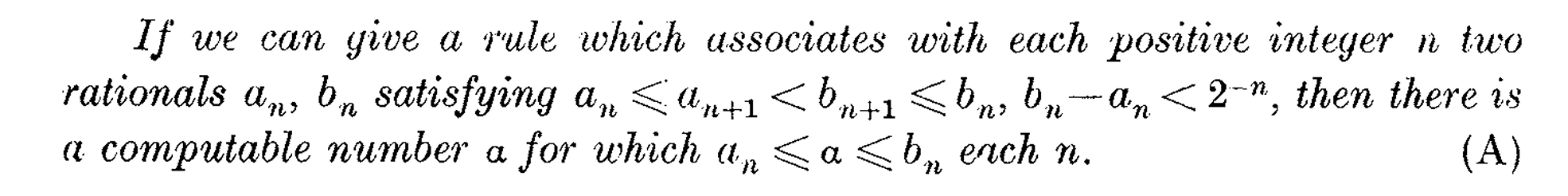
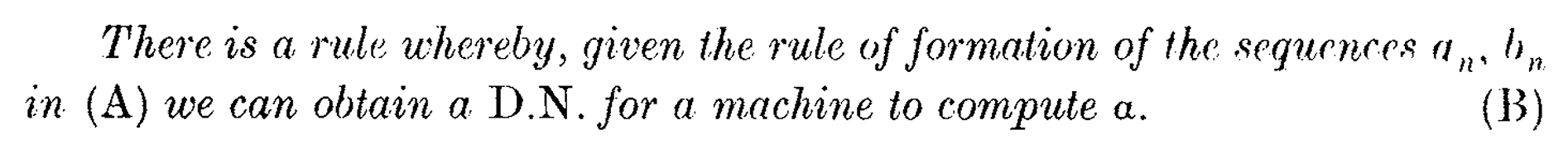
Rewritten in modern terminology, Turing hopes that whatever rule we adopt for defining a computable real number would satisfy the two properties:

In his correction, Turing notes how (A) holds for his original characterization of computability for real numbers under a proof by contradiction (axiomatically, the Law of Excluded Middle). Having the ability to uniformly compute a \((2^{-n})\)-rational-approximation to a real without the real being computable means the real has to have a tail of all \(1\)'s begin somewhere in its expansion, making it computable after all.

The more important observation comes from (B): Turing first notes that (B) is false in his original formalization of computable reals that associates them to infinite binary strings which never terminate in infinite tails of \(1\)s. Assuming (B) to be true, he constructs an example pair of sequences satisfying (A) for an arbitrary fixed Turing Machine \(\mathcal{M}\) which was used to compute both sequences, but proves how the computable \(\alpha\) guaranteed by (A) would necessarily have its first bit able to decide the question: "Does \(\mathcal{M}\) ever output a zero on its own tape during the course of its computation?" This property is known to be undecidable in \(\mathcal{M}\); that is, at the same level as the Halting Problem/Entscheidungsproblem relative to \(\mathcal{M}\) when \(\mathcal{M}\) is an arbitrary Turing Machine. This is a contradiction to the supposed computability of \(\alpha\).

In response, Turing offers a workaround to this "disagreeable situation": a computable binary sequence of the following format can be associated to the corresponding real:

\[c_0 1^n 0 c_1 c_2 \cdots \quad \rightsquigarrow \quad (2 c_0 - 1) n + \sum_{r = 1}^\infty (2 c_r - 1) \left(\frac{2}{3}\right)^r.\]

Call the reals associated to at least one computable, infinite binary sequence of this form to be computable themselves. The intervals/jumps used in this sum are "fat" in the sense that jumps at one level \(r\) can undo jumps from previous levels, meaning there is significant overlap in the effects of various \(c_i\) in how they affect the associated real's value. This introduces a higher degree of non-injectivity/non-uniqueness to representing reals. Turing comforts the reader that this sacrifice is of no serious preoccupation: Turing Machines are already represented by infinitely many algorithms/programs/Machine codes.

Turing explains that now (B) is satisfied under the new association: because we know that our computable \(\alpha\) is the unique element of the singleton set \(\{\alpha\} = \bigcap_{n \in \mathbb{N}} [a_n, b_n],\) it is easy to see that we can easily deduce the first \(r\) many values \(c_r\) in the associated infinite binary sequence to \(\alpha\) by looking sufficiently far into the sequence of \((a_n)\) and \((b_n)\): just make sure that the jump of length \(\left(\frac{2}{3} \right)^{r}\) exceeds the approximation size \(2^{-n}\). This will force us to assign values to all \(c_k\) with \(k \leq r\). This process is algorithmic, and so we have a uniform way to take a uniform description for the sequences \((a_n), (b_n)\) to a description for a machine that outputs \(\alpha\).

With this in mind, allow us to proceed to further generalizations.

Miller's Answer

In 2014, Joseph Miller published Degrees of Unsolvability of Continuous Functions, where he fixes a notion of representation (what I will call a name) which is general enough to work for any computable metric space (Miller 2014). As we will see, because the real numbers will satisfy the definition of a such a space, we will have a new way of representing the real numbers and working on them computability-theoretically. This method, when applied to the real numbers, provides an equivalent notion to what Turing's corrected association does, so we have great agreement amongst our various adopted characterizations of computability.

Define a computable metric space (definition due to (Lacombe 1959)) to be a tuple \((\mathcal{M} ; d_{\mathcal{M}} : \mathcal{M} \times \mathcal{M} \to \mathbb{R}_{\geq 0} ; \mathcal{Q}^{\mathcal{M}} = \{q^{\mathcal{M}_n}_{n \in \mathbb{N}} \subseteq \mathcal{M}\})\) such that \(\mathcal{Q}^{\mathcal{M}}\) is a computable, dense subset of \(\mathcal{M}\) and such that \(d_{\mathcal{M}}\) restricted to \(\mathcal{Q}^{\mathcal{M}}\) is a computable function. This last condition formally means there exists a computable function \(\delta: \mathbb{N}^2 \times \mathbb{Q}^2 \to \mathbb{Q}\) such that for any \(i, j, \varepsilon\),

\[\left| \delta(i, j, \varepsilon) - d_{\mathcal{M}}\left(q^{\mathcal{M}}_i, q^{\mathcal{M}}_j \right)\right| < \varepsilon.\]

This notation seems rather abstract, but I suggest understanding it as follows:

• \(d_{\mathcal{M}}(x, y)\) is the distance function between the numbers: its analogy in the reals is the Euclidean distance \(\left|x - y\right|\).
• \(\mathcal{Q}^{\mathcal{M}}\) is a computable dense set within the space that will be used to determine the computability of the remaining numbers: its analogy in the reals is \(\mathbb{Q}\), which is both dense and consisting of only computable numbers.
• Computability of \(d_{\mathcal{M}}\) is like asking that detecting the difference between two rational numbers is a computable process. Surely this is true: it's simple subtraction that doesn't require any approximation when we evaluate it on just rationals.

In order to define computability for elements of the space, we only cosmetically edit the second idea from the first section:

Example: \((\mathbb{R} ; \left| \cdot \right| ; \mathbb{Q})\) is a computable metric space, as described in the bullets above. We claim that the computability notion coming from viewing \((\mathbb{R} ; \left| \cdot \right| ; \mathbb{Q})\) as a computable metric space (a.k.a., Miller's sense) matches precisely the standard computability notion described by, say, Turing. Notice that in order to be computable in Miller's sense, a real number must have a name \(\lambda: \mathbb{Q}_{ > 0} \to \mathbb{N}\) satisfying \(\left | x - q_{\lambda(\varepsilon)}\right| < \varepsilon\) for all \(\varepsilon \in \mathbb{Q}_{> 0}\) and which is computable. This is equivalent to asking there exist a single Turing Machine or algorithm \(\Phi_e : \mathbb{Q}_{> 0} \to \mathbb{Q}\) which can approximate \(x\) up to any positive, rational precision. This matches with Turing's notion of computability for reals. This correspondence between the two notions is no accident: Miller's general definitions were inspired by the previous decades of work already done on these prototypical computable metric spaces.

Furthermore, when mapping between two computable metric spaces \(\mathcal{M}_0, \mathcal{M}_1\), a function \(\psi: \subseteq \mathcal{M}_0 \to \mathcal{M}_1\) is called partial computable if there exists \(e \in \mathbb{N}\) such that the \(e\)-th oracle Turing Machine \(\Phi_e\) induces \(\psi\); that is: for any name \(\lambda\) of \(x \in \mathcal{M}_0\):

\[\left(\psi(x) \downarrow \longrightarrow \Phi^\lambda_e \text{ names } \psi(x) \in \mathcal{M}_1 \right) \text{ and } \left(\psi(x) \uparrow \longrightarrow \Phi^\lambda_e \text{ is not total} \right)\]

In particular, being partial computable means having a Turing Machine which mimicking its outputs when given the name of an input, but also failing to converge wherever \(\psi\) is undefined.

As a particular case, we call such partially computable \(\psi: \mathcal{M}_0 \to \mathcal{M}_1\) (total) computable if its domain is all of \(\mathcal{M}_0\).

We claim, as an extension to the previous example for the real numbers, that a real-valued function \(f\) on \(\subseteq \mathbb{R}\) is (partial) computable in the sense of Miller iff it is so in the classical sense. To see this, note that partial computability in Miller's sense here means that there exists \(e \in \mathbb{N}\) such that for any name \(\lambda\) of \(x \in \mathbb{R},\) then

\[\left(f(x) \downarrow \longrightarrow \Phi^\lambda_e \text{ names } f(x) \in \mathbb{R} \right) \text{ and } \left(\psi(x) \uparrow \longrightarrow \Phi^\lambda_e \text{ is not total} \right).\]

Equivalently, that is to say that if we have an algorithmic way to compute a rational arbitrarily close to \(x \in \mathbb{R}\) then we should have a uniform algorithm (provided an oracle for \(x\)) for which: either \(f(x) \downarrow\), in which case our algorithm can be able to produce an arbitrarily close rational approximation to \(f(x)\), or \(f(x) \uparrow\), in which case our uniform algorithm should fail to produce any approximation to \(f\) by diverging. This is exactly what is meant by \(f\) being partial computable in the usual sense.

A typical way you may see computability defined for real functions is as follows:

This definition should be equivalent to Miller's on \(\mathbb{R}\): oracles play a similar role to names, but are of a slightly different type: \(\mathbb{N} \to \mathbb{Q}\) versus \(\mathbb{Q}_{> 0} \to \mathbb{N}\). Luckily, all of these sets are effectively enumerable, so fixing some effective enumeration of each, they are, up to some effective encoding, of the same type. Moreover, names technically output indices of elements from \(\mathcal{Q}^{\mathcal{M}}.\) For us, that set is \(\mathbb{Q}\). So again, after fixing an effective enumeration, the two notions are of the same type. The only difference is that oracles work only on the error sequence \((2^{-r})_{r \in \mathbb{N}}\), whereas names use any \(\varepsilon \in \mathbb{Q}_{> 0}.\) As it turns out, this difference in choice does not lead to any difference in which functions get labeled computable, for any name \(\lambda\) of \(x\) can effectively produce an oracle \(g\) of \(x\) by setting \(g(n) := q_{\lambda(2^{-n})}\), and vice versa by \(\lambda(\varepsilon) := \operatorname{index}_{\mathbb{Q}}\left(g\left( 2^{-(n + 1)} \right)\right).\)

Conclusion

For my purposes, it will be worth the effort to consider all of my computability statements in this general framework rather than using the intuitive "compute the first \(n\)-bits" explanation, especially to avoid its non-uniformity at dyadic rationals. And it might be the case that some of my results apply to these general computable metric spaces rather than just Euclidean space. For all of these reasons, I offer you all this introduction to to the Theory of Representations within Computability Theory/Algorithmic Information Theory. Thank you!

Bibliography

• (Lacombe 1959) Daniel Lacombe. Quelques procédés de définition en topologie recursive. 1959.
• (Miller 2014) Joseph S. Miller. Degrees of Unsolvability of Continuous Functions. 2014.
• (Turing 1936) A. M. Turing. On Computable Numbers, with an Application to the Entscheidungsproblem. 1936.
• (Turing 1937) A. M. Turing. On Computable Numbers, with an Application to the Entscheidungsproblem – A Correction. 1937.